Factor Exposure Analysis 111: What is Alpha?

Comparing different alpha calculation methodologies

March 2025. Reading Time: 10 Minutes. Author: Abhik Roy, CFA.

SUMMARY

Jensen’s alpha methodology is popular, but has several drawbacks
There is no perfect methodology, but some are more easy to understand than others
We prefer the residual return (beta-adjusted excess return) approach given its robustness and simplicity

INTRODUCTION

Since Michael Jensen formalized the concept of alpha in his 1968 paper, The Performance of Mutual Funds in the Period 1945-1964, it quickly became a key metric for fund managers to measure their ability to outperform the market, driving its widespread adoption.

However, Eugene F. Fama and Kenneth R. French later introduced their three-factor model, demonstrating that alpha often diminishes when portfolio returns are adjusted for three key factors: market, size, and value. Over time, additional factors have been identified, further explaining excess returns and reducing the magnitude of alpha (read Outperformance Ain’t Alpha).

But a lot of these models may seem too theoretical, which can then lead to investors questioning the practicality of the metric. In this research, we will compare different methods for calculating alpha.

ALPHA AS THE INTERCEPT

As per the initial paper by Michael Jensen, “alpha” was calculated based on Capital Asset Pricing Model (CAPM), taking the intercept of the regression as alpha, while beta became the measure of systematic risk. The frequency of the data used were annual. Below is an excerpt from the paper:

Factor Betas of Long-Only Factor Portfolios Portfolio Concentration

Source: The Journal of Finance, “The Performance of Mutual Funds in the Period 1945-1964”.

Although the above calculation seems straightforward, applying it to real world data poses some challenges:

The model considers only market risk, without accounting for other factors that may influence excess portfolio returns. As the CAPM framework evolved, additional factors were identified that better explain performance variations.
The model does not give visibility into the dynamically changing allocations of the portfolio.
Funds often don’t have sufficient history. According to Morningstar, the average lifespan of active ETFs closed in 2023 was just 2.6 years, while passive ETFs averaged 5.9 years. This limited data availability makes it difficult to derive reliable regression coefficients.
Interpreting the actual inference from the metric is often difficult for non-statisticians.

FINDING AN ALTERNATIVE

To address these limitations, we change the calculation methodology. Specifically, we incorporate additional factors—value, quality, low volatility, momentum, and size—alongside market risk. In addition, we reduce the frequency of data to weekly, so we can calculate the regression statistics for each year.

We will now evaluate four different methods for calculating alpha. To do this, we select a sample of 10 equity-focused funds and compare the alpha values derived from each method to the original alpha calculated using Jensen’s model, adjusted for additional factors.

Beta Adjusted Excess Return – Average: We calculate alpha by subtracting the beta-adjusted factor returns from the fund’s return for each calendar year. We then aggregate these alpha values over the fund’s entire history to determine the overall alpha.
Intercept Scaled – Average: Here, we estimate alpha for each calendar year as the intercept of the regression for that year. We then adjust it using an annualizing factor and compute the average alpha across all calendar years for the fund as mentioned below:

Factor Betas of Long-Only Factor Portfolios Minimum Market Cap Thresholds ($ billions)

Intercept Scaled: This method follows the same approach as the Intercept-Scaled – Average method but instead of calculating alpha separately for each calendar year and averaging the results, we use the fund’s entire return history to estimate a single alpha. The calculated alpha is then annualized using the adjustment from Step 2.
Beta-Adjusted Excess Returns – Annualized: In this method, we calculate alpha by first determining the annualized mean return of the portfolio for each calendar year. We then subtract the beta-adjusted annualized factor returns for the same period. Finally, we average these yearly alpha values over the fund’s history.

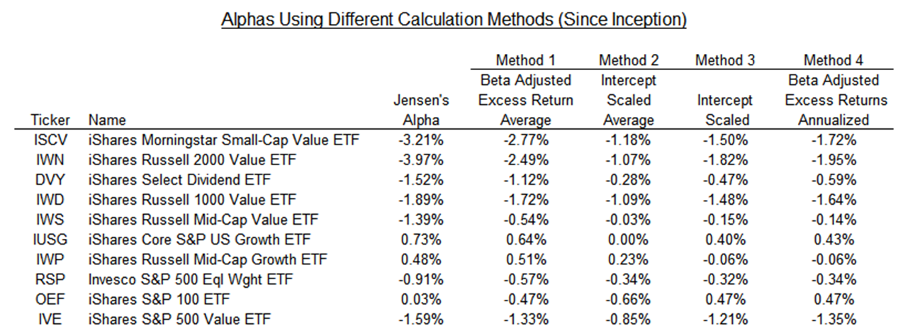
Below are the results from the various calculation methods. As expected, different methodologies yield different alpha values, highlighting the impact of calculation choices. This raises an important question: Which method provides the most accurate and meaningful measure of alpha?

Multifactor Model Top 30% Market Cap-Weighted versus Top 10% Equal-Weighted

Source: Finominal

An ideal measure of alpha should address all the limitations discussed previously and closely align with the true Jensen’s Alpha. Among the methods, Beta-Adjusted Excess Return – Average (Method 1) stands out because it can be easily interpreted as the residual return after beta-adjusted factor returns. In contrast, the other methods involve scaling, which diminishes their interpretability.

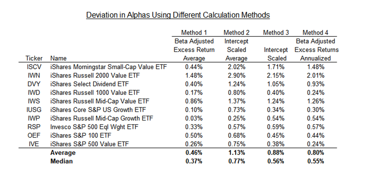
To assess how well each method approximates Jensen’s Alpha, we measure the absolute deviations for all the funds and compare the average deviation. As shown in the table below, we find that Beta-Adjusted Excess Return – Average (Method 1) produced the smallest deviation, followed by methods 4, 3, and 2.

Source: Finominal

FURTHER THOUGHTS

Given both interpretability and deviation, Beta-Adjusted Excess Return – Average (Method 1) emerges as the most suitable approach for calculating alpha for any fund or portfolio. This method effectively addresses the limitations of Jensen’s Alpha, producing the smallest deviations while maintaining clarity in its interpretation.

While many other techniques may exist to calculate alpha, investors should find it understandable and be able to infer actionable insights. This idea is aptly summarized by the British statistician George Box: “All models are wrong, but some are useful.”

RELATED RESEARCH

ABOUT THE AUTHOR

Abhik Roy, CFA is a Quantitative Researcher at Finominal, which empowers professional investors with data, technology, and research insights to improve their investment outcomes. Abhik holds a Masters in Economics and Bachelors in Engineering from BITS Pilani. Previously he worked at Kristal.AI, a Singapore based fintech firm as a Quantitative Analyst.

Connect with me on LinkedIn .