Factor Exposure Analysis of Fixed Income ETFs

What is driving the risk & return of bond strategies?

June 2022. Reading Time: 10 Minutes. Author: Nicolas Rabener.

SUMMARY

• Factor exposure analysis can be used in fixed income as easily as in equities
• More variables improve the explanatory power of the model
• However, it also can make the interpretation challenging

INTRODUCTION

Running a factor exposure analysis is a core element of the due diligence process for equity-focused mutual funds, and increasingly ETFs, especially actively managed ones. The holy grail is to find fund managers that generate outperformance that is not explained by equity factors, ie alpha. If excess returns can be explained by factor exposure, then the capital allocator can simply pick a smart beta ETF with the same factor exposure at a lower cost.

However, although it has the same relevance, a factor exposure analysis is slightly less frequently used when evaluating fixed income strategies. Perhaps this is explained by bonds seeming to be more complicated than equities. There is only one type of equities, compared to several types of fixed income instruments that range from convertible debt to senior loans.

Furthermore, there is less consensus on how to define factors in fixed income than in equities. Although there are no exact standards on how to calculate the value or quality factors for stocks, most researchers look at the academic work of Fama-French for guidance. There is no equivalent standard for fixed income (read The Complexity of Factor Exposure Analysis).

In this research note, we explore some of the practical questions when running a factor exposure analysis for fixed income strategies.

SELECTION OF FIXED INCOME STRATEGIES

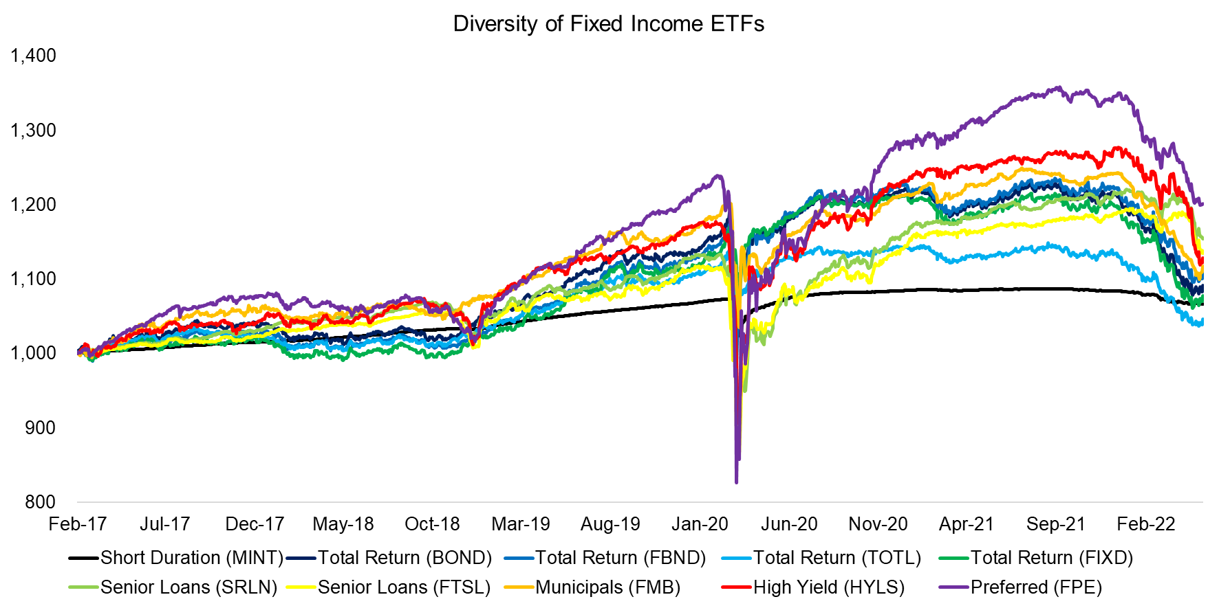
We select 10 actively managed fixed income ETFs traded in the US, of which the oldest has a track record going back to 2009. The management fees range from 0.35% to 1.13%, and the cumulative assets under management are $48 billion.

The strategies are quite diverse and provide exposure to low-risk short-term US government bonds as well as riskier high yield bonds. The performance over the last five years highlights the diversity as the total return ranges from 3.9% to 20.1% (read Smart Beta Fixed Income ETFs). 

Source: FactorResearch

FACTOR EXPOSURE ANALYSIS OF BONDS

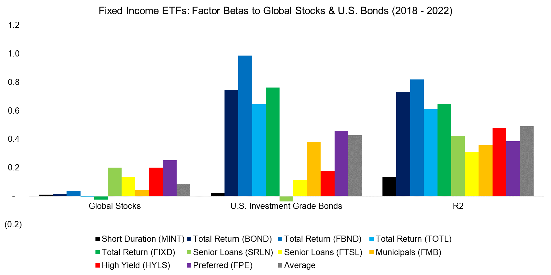
Some of the products are labeled total return strategies, which is not self-explanatory for understanding what kind of bond exposures these provide. We initiate the factor exposure analysis by using only two independent variables namely global stocks and U.S. investment grade bonds and calculate factor betas using five years of daily data.

The analysis highlights that some of the strategies had minor exposure to equities and only half had high exposure to U.S. investment grade bonds, which is perhaps less than expected. One of the senior loan ETFs had negative exposure to bonds but moderate equity exposure, which shows that senior loans may provide fewer diversification benefits for an equity portfolio than other fixed income instruments (try Finominal’s Alpha Analyzer for a factor exposure analysis).

Source: FactorResearch

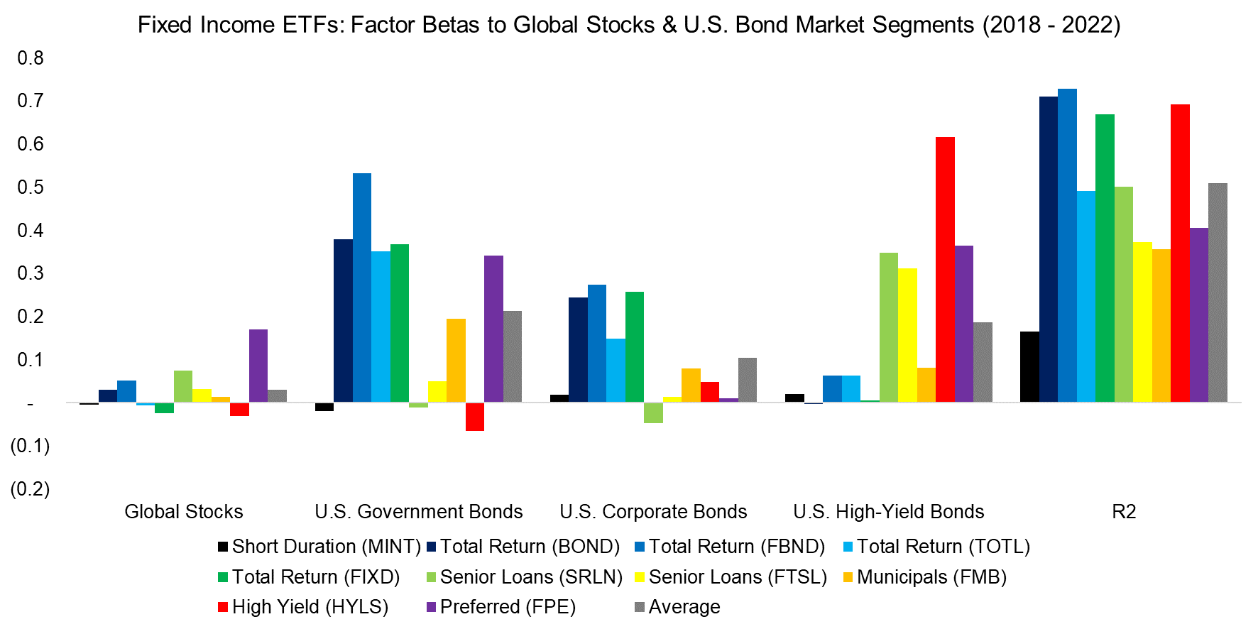
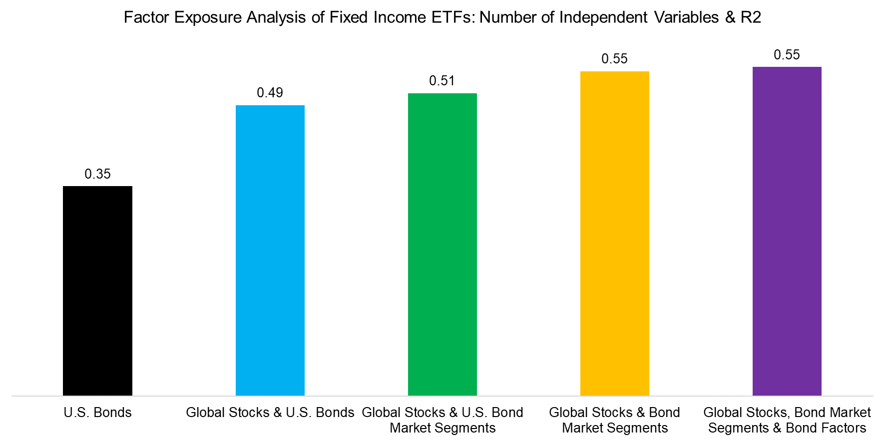
However, the average R2 was only 0.5, which indicates that the explanatory power of the regression analysis is not particularly high. In order to increase this, we replace the U.S investment grade bond index with three indices representing U.S. government, corporate, and high yield bonds.

We observe that the average R2 does not increase by including more variables and remains at 0.5. However, the results are more nuanced and also intuitive, eg the returns of the high yield ETF can be attributed to the performance of high yield bonds. 

Source: FactorResearch

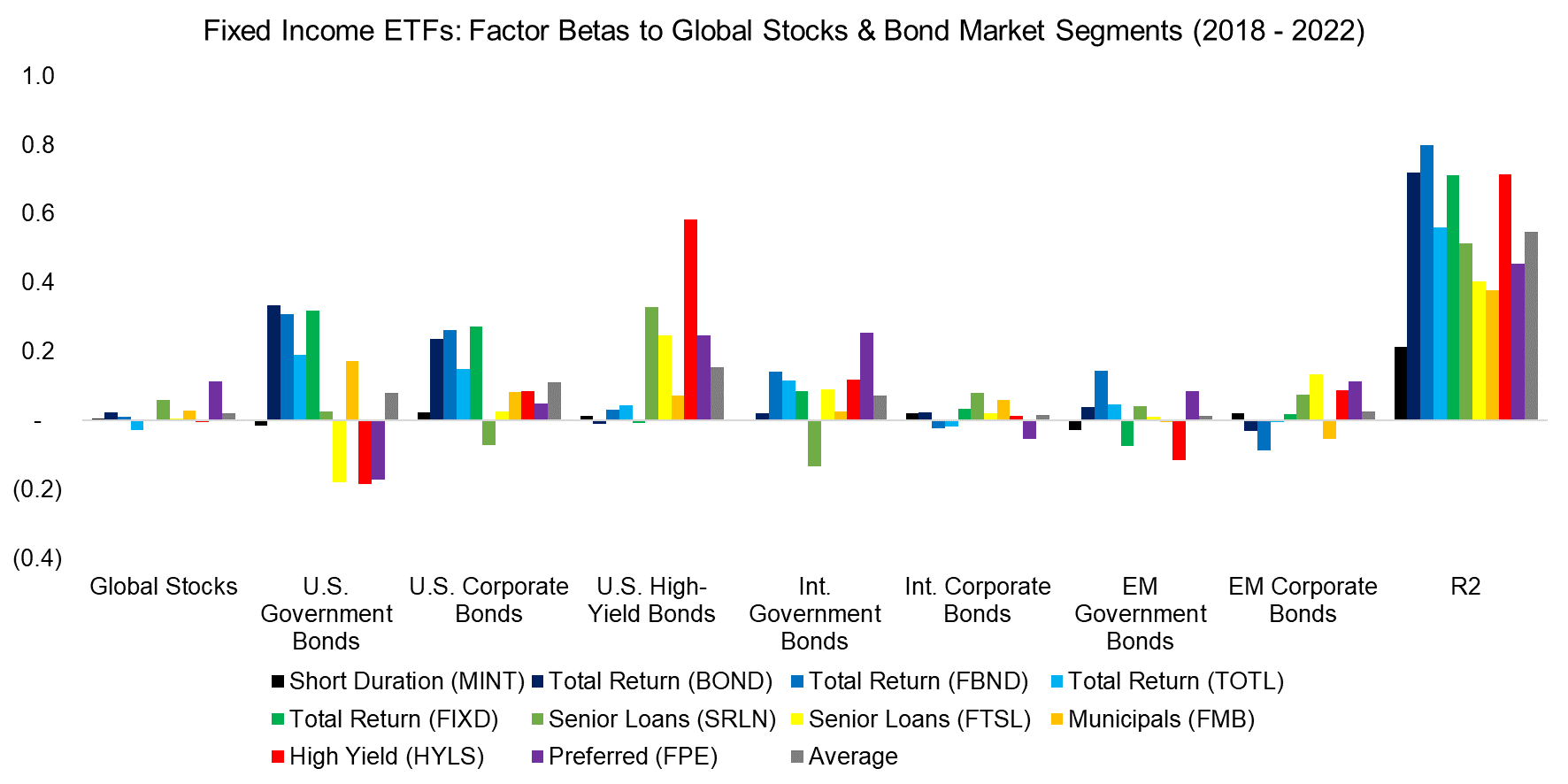
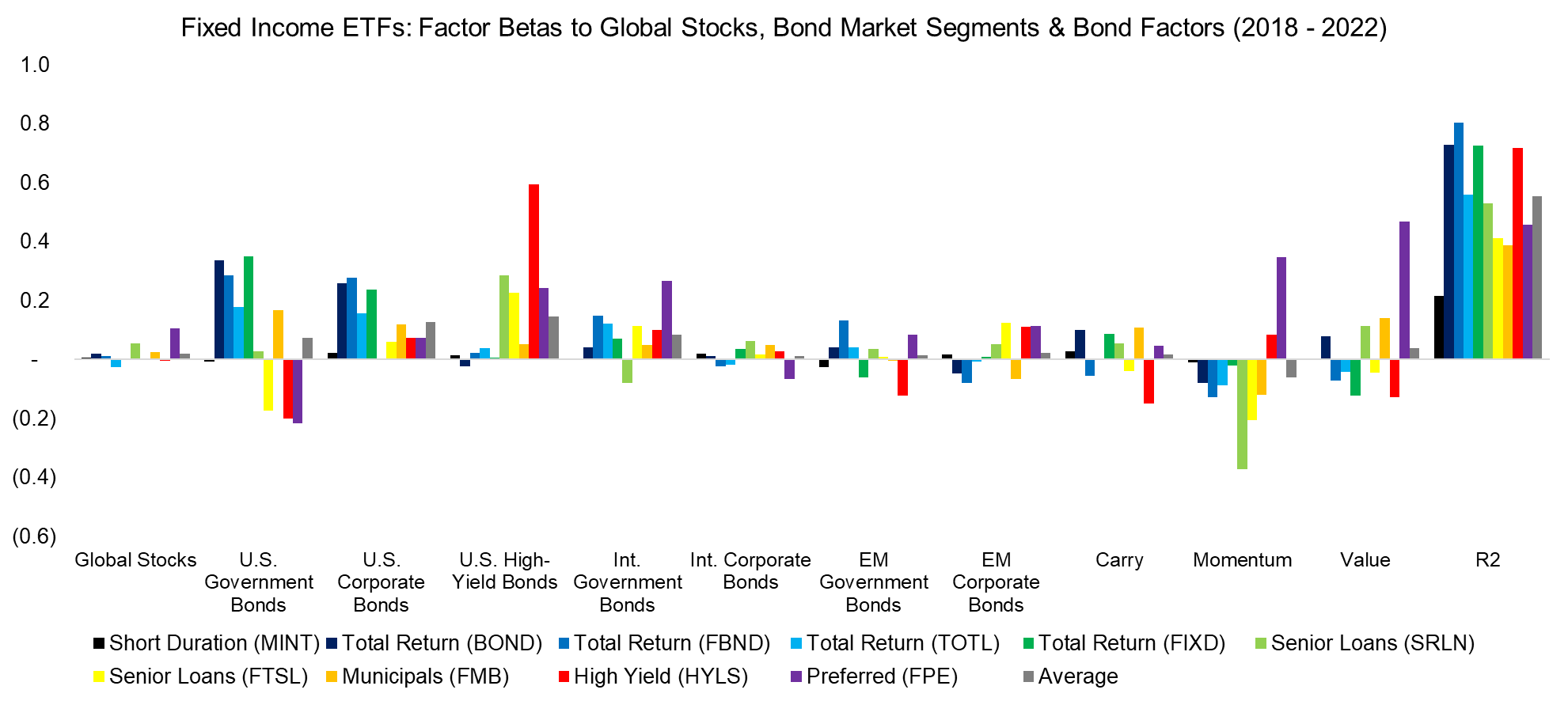
Next, we increase the number of independent variables further and include international and emerging bond indices. We now have one equity and seven bond indices.

The average R2 increases from 0.51 to 0.55, but interpreting the results starts to become more challenging. For example, the high yield ETF has positive exposure to U.S. high yield bonds, but negative exposure to U.S. and emerging market government bonds. The latter is somewhat unusual as emerging market government and U.S. high yield bonds tend to have positive correlations, ie the factor beta should be positive rather than negative.

Source: FactorResearch

As a final step, we add three bond factors namely carry, momentum, and value, so use a total of 11 indices. The average R2 does not increase further and remains at 0.55. 

We observe that the actively managed ETFs did have factor exposures, which need to be considered when calculating their outperformance via their benchmarks. However, in contrast to equites, the universe of fixed income smart beta ETFs is small. Even if investors are able to explain that outperformance can be attributed to factors rather than skill (alpha), they can not easily replace the fund manager with a smart beta ETF.

Source: FactorResearch

NUMBER OF INDEPENDENT VARIABLES 

Although the average R2 did not increase significantly by adding more indices, it did marginally and allows investors to attribute returns to the different types of fixed income instruments, as well as different geographies. Essentially, the factor exposure analysis creates transparency on what has been driving the risk and return of strategies, which might not always be appreciated by the fund manager.

Source: FactorResearch

FURTHER THOUGHTS

The analysis can be easily challenged as we only used the R2 to judge the results and have not shown the p-values. However, these two are closely related and the p-values have also improved as more variables were added. The next logical step would be to use a Lasso regression or similar methodology that selects only the most relevant variables and ignores the rest.

It is easy to contemplate having hundreds of variables so the return of a strategy can be fully explained, but there are not that many independent variables, and even using machine learning to sort through these is not always helpful. Some of the factor exposures are not particularly easy to explain, where it is difficult to decide if this exposure uncovers a new relationship, or is statistical junk. The more variables the better, but only to a degree.

RELATED RESEARCH

Analyzing Floating Rate ETFs
Factor Exposure Analysis: Exploring Residualization
Time Machines for Investors
Musings about Factor Exposure Analysis
Factor Exposure Analysis 101

ABOUT THE AUTHOR

Nicolas Rabener is the CEO & Founder of Finominal, which empowers professional investors with data, technology, and research insights to improve their investment outcomes. Previously he created Jackdaw Capital, an award-winning quantitative hedge fund. Before that Nicolas worked at GIC and Citigroup in London and New York. Nicolas holds a Master of Finance from HHL Leipzig Graduate School of Management, is a CAIA charter holder, and enjoys endurance sports (Ironman & 100km Ultramarathon).

Connect with me on LinkedIn or Twitter.