Mean-Reversion Across Markets

Hedging Tail Risks of Equity Portfolios

May 2018. Reading Time: 10 Minutes. Author: Nicolas Rabener.

SUMMARY

The Mean-Reversion factor shows the same trends across markets
The strategy differentiates itself from other factors by exhibiting strong positive skewness
Mean-Reversion is an attractive diversifier for an equity-centric portfolio

INTRODUCTION

Volatility spiked in the first quarter of 2018 when global stock markets declined, which was mainly due to concerns on proposed tariffs by the US government and rising interest rates. Since then markets recovered and volatility declined again, but higher interest rates are likely to have a negative impact on the global economy given record levels of public, corporate and consumer debt. Higher rates probably result in lower corporate earnings and decreased consumer spending, which would lead to markets performing less well than in recent years and volatility to increase. Although this scenario would be a concern for most investors with traditional equity-bond portfolios, there are some strategies like Mean-Reversion that benefit from higher levels of volatility. In this short research note we will analyse the performance and characteristics of the Mean-Reversion factor and its potential utilisation in an equity-centric portfolio (read Death, Taxes and Mean-Reversion).

METHODOLOGY

We focus on the Mean-Reversion factor in the US, Europe and Japan. The factor is created via dollar-neutral long-short portfolios buying stocks with the worst weekly returns and shorting stocks with the highest weekly returns. The portfolios are created daily and rebalanced weekly, which results in a strategy with an exceptionally high turnover. In the US the top and bottom 2.5% of the stock universe are selected for the portfolio construction compared to the top and bottom 5% in Europe and Japan. Only stocks with a market capitalisation of larger than $1 billion are included. Transaction costs of 5 basis points are assumed for the US and 10 basis points for Europe and Japan.

MEAN-REVERSION ACROSS REGIONS

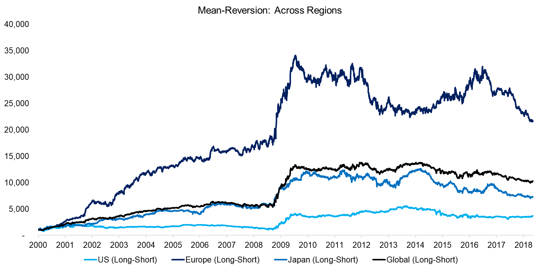
The chart below shows the performance of the Mean-Reversion factor in the US, Europe, Japan and globally, which equally allocates to these three markets, from 2000 to 2018. Overall the profiles are quite similar, which highlights that the factor likely has the same underlying drivers. The factor performance has been significantly higher in Europe and Japan than in the US, which might be explained by less competition or by the backtesting assumptions. The strategy is highly sensitive to transaction costs given high turnover, so the results should be regarded with caution. Compared to other factor strategies, investors can expect a higher discrepancy between theoretical and realised returns (read Mean-Reversion on Equity Index Level).

Source: FactorResearch

MEAN-REVERSION IN THE US

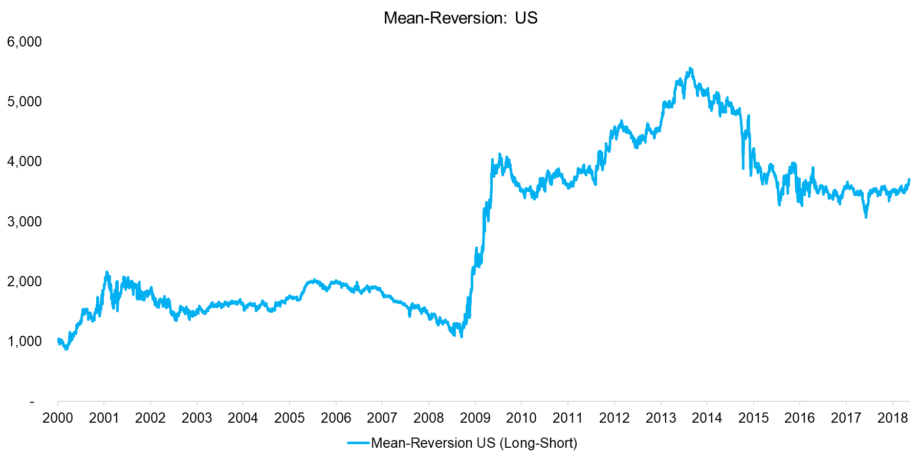
The performance of Mean-Reversion in the US seemed somewhat flat compared to Europe and Japan, but was positive since 2000 as highlighted by the chart below. However, almost 50% of the performance can be attributed to a few months in 2008 and 2009 and there were multiple years of flat and declining returns, which makes this strategy challenging for fund managers and capital allocators.

Source: FactorResearch

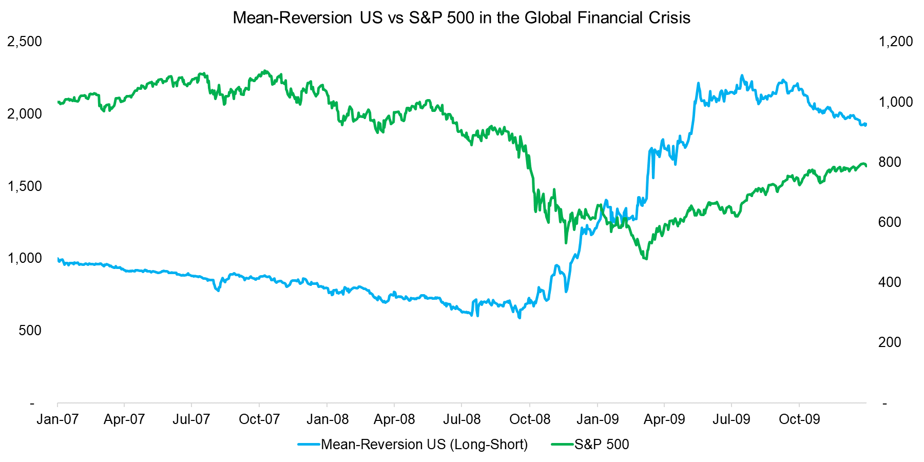
It is interesting to analyse the performance of the Mean-Reversion factor in 2008 and 2009, given that this period contributed almost the majority of the returns over the last two decades. Naturally this period represents the Global Financial Crisis, where the S&P 500 experienced a drawdown of more than 50%. The chart below compares the performance of the factor and the S&P 500 and we can observe that both declined consistently from 2007 to the middle of 2008. However, in September 2008 the performance started diverging with Mean-Reversion generating substantial gains while the S&P 500 deteriorated further. The analysis highlights that a declining market does not necessarily lead to positive returns from the Mean-Reversion factor.

Mean-Reversion US vs S&P 500 in the Global Financial Crisis

Source: FactorResearch

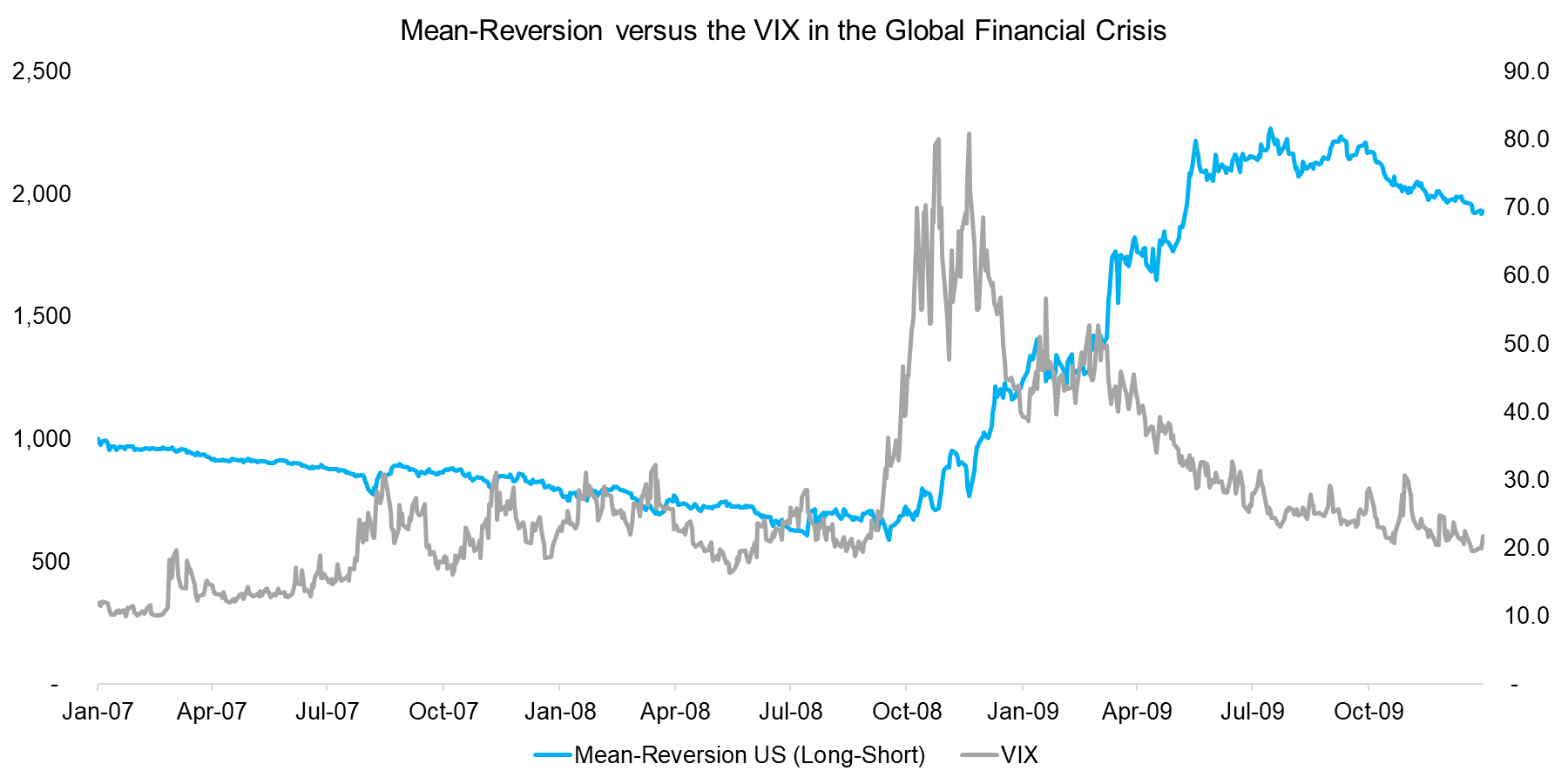
In addition to comparing the performance of the Mean-Reversion factor to the S&P 500, we can also display the VIX, which represents implied volatility. The chart below highlights that the Mean-Reversion factor started generating substantial returns above a VIX level of 20, which was reached in September 2008 after Lehman Brothers declared bankruptcy and investors started questioning the financial health of most major banks. During that period investors likely overreacted and mispriced stocks frequently, which is the main source of profits for a liquidity-providing strategy like Mean-Reversion. The analysis also shows that the factor performance deteriorated once volatility started declining when stock markets recovered in 2009.

Mean-Reversion versus the VIX in the Global Financial Crisis

Source: FactorResearch

CHARACTERISTICS OF THE MEAN-REVERSION FACTOR

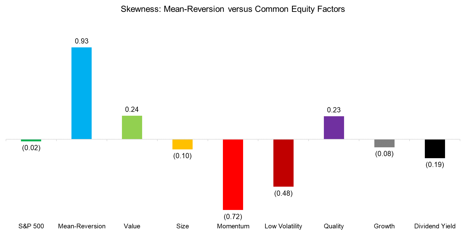
The Mean-Reversion factor differentiates itself from most other common equity factors by exhibiting significantly positive skewness, which describes that the return distribution includes some extreme positive gains. The chart below highlights that the returns of the S&P 500 were not skewed for the period from 2000 to 2018, while the Momentum factor (long-short) exhibited significantly negative skewness. It is worth highlighting that holding a portfolio with negative skewness is emotionally difficult as it implies long periods with flat or slightly declining performance. Therefore strategies like Mean-Reversion or cross-asset class trend following, which also exhibits positive skewness, should be considered as satellite strategies within a larger portfolio and acknowledged for their rare, but useful contributions to the portfolio.

Skewness Mean-Reversion (Long-Short) versus the S&P 500

Source: FactorResearch

MEAN-REVERSION IN AN EQUITY-CENTRIC PORTFOLIO

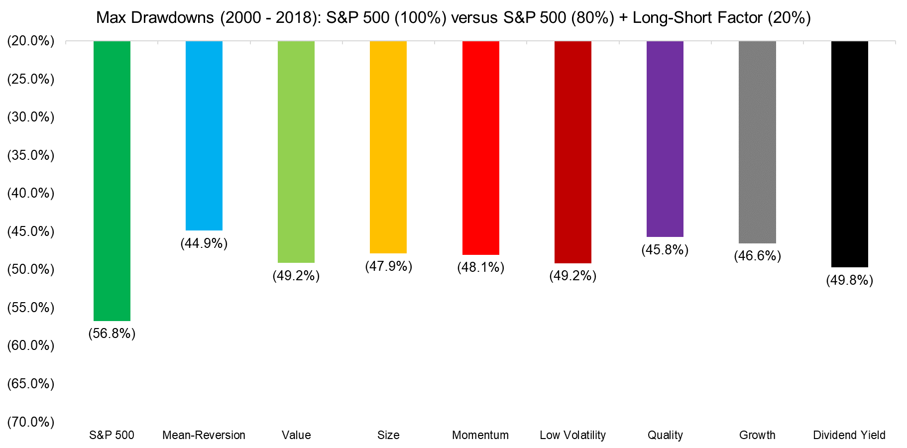
Given that the Mean-Reversion factor exhibits positive skewness and tends to generate substantial profits when markets decline and volatility is high, it should be an interesting addition to an equity-centric portfolio. The analysis below displays the maximum drawdowns of portfolios that consist of the S&P 500 (80% allocation) and a variety of long-short factors (20% allocation). As expected all combination portfolios show a reduced maximum drawdown compared to the S&P 500 on a stand-alone basis, but the portfolio that includes Mean-Reversion results the highest reduction.

Skewness Mean-Reversion versus Common Equity Factors

Source: FactorResearch

FURTHER THOUGHTS

This short research note highlights the performance and characteristics of the Mean-Reversion factor, which is an attractive addition for an equity-centric portfolio. Unfortunately the unique nature of this strategy makes it less attractive for most investors as high turnover is often considered a negative for investment strategies and positive skewness implies long periods of flat or declining returns. Given that the factor is mainly driven by volatility, investors could consider a tactical versus strategic allocation, although that would require either discretionary or systematic timing skills (try Finominal’s Volatility Optimizer for risk optimization).

ABOUT THE AUTHOR

Nicolas Rabener is the CEO & Founder of Finominal, which empowers professional investors with data, technology, and research insights to improve their investment outcomes. Previously he created Jackdaw Capital, an award-winning quantitative hedge fund. Before that Nicolas worked at GIC and Citigroup in London and New York. Nicolas holds a Master of Finance from HHL Leipzig Graduate School of Management, is a CAIA charter holder, and enjoys endurance sports (Ironman & 100km Ultramarathon).

Connect with me on LinkedIn or Twitter.